Gaussian Pulse in Pressure in a Cube

In this example, we will simulate a Gaussian pulse in pressure in a simple pre-defined cube with periodic boundaries and user-defined initial condition. The gaussian pulse can be also used via a pre-defined function, c. f. * pre-defined gaussian pulse For this simple geometry, we even do not need Seeder.

The objectives of this example is to introduce how to: * Use a pre-defined geometry instead of creating a mesh with Seeder. * Simulate the Gaussian pulse in the cube using Musubi. * Create 2D plots using the Gleaner tool. Gleaner is a Python tool that extracts data from Musubi ASCII output and uses the plotting library Matplotlib in Python to create a plot. * Validate the numerical results by comparing them against the analytic solution. The latter one is calculated using NumPy, a mathematic extension for Python. * Compare the simulation results (L4) to previously generated data obtained with higher resolution (reference folder, L5 & L6) to experience the influence of the resolution.

ToDo

This file has to be filled with content like: * Problem description * Formulas * Results * Comparison for different resolutions * How to run the simulation

Here are the results from the simulation.

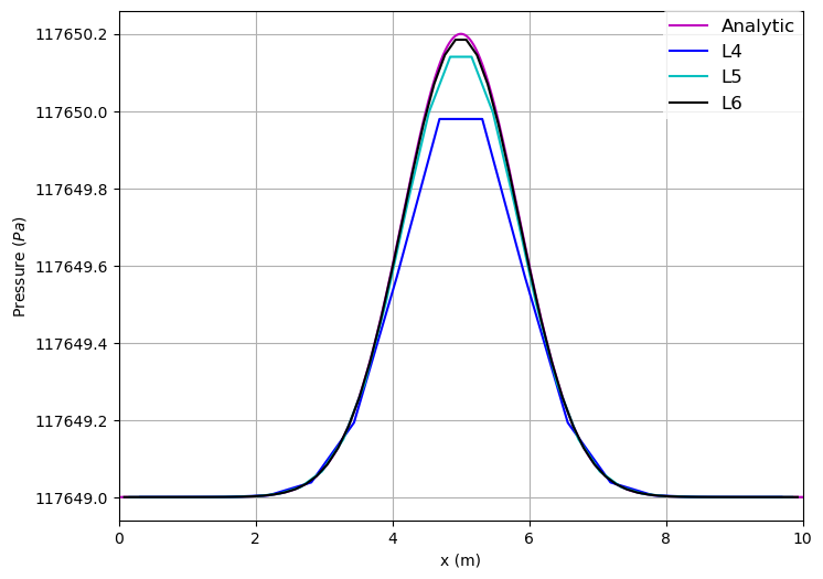
Pressure across the length of the channel for different resolutions at the beginning (initial condition): Pressure_Profile-IC The higher the level -- and with that the resolution -- the better the solution compared to the analytical one.

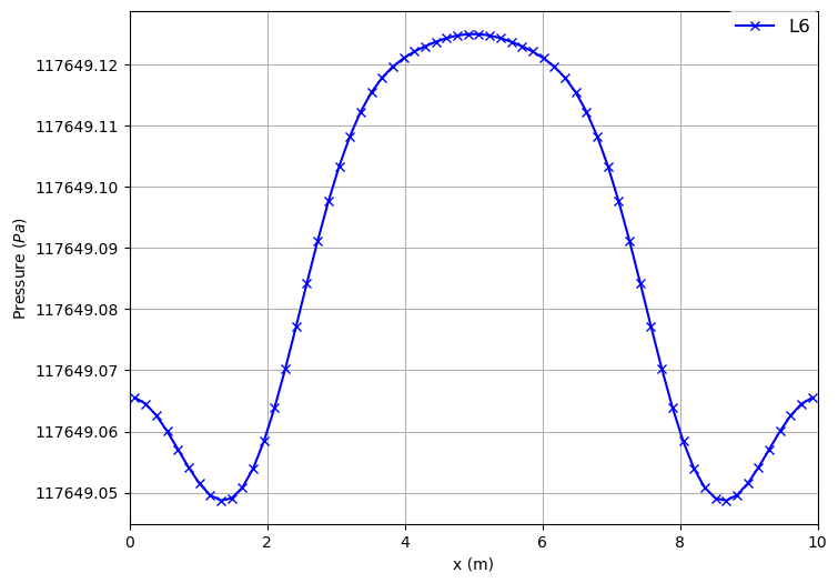
Pressure across the length of the channel for high resolution (L6) at the end: Pressure_Profile To reproduce this plot, set 'shepherd = false' in musubi.lua.

To create these plots, run python plot_track.py to create the plots. Before running the plot script, open 'plot_track.py' and update path to Gleaner script in 'glrPath'. Download Gleaner script using hg clone https://geb.sts.nt.uni-siegen.de/hg/gleaner

Documentation Bibliography Examples Weakly compressible flows Applications Nonreflecting Boundary Conditions Nozzle Nozzle flow inside an around Nozzle flow inside Benchmarks Channel 2D Channel 2D Boundary Conditions Channel 2D MfrBB PressExpol Channel 2D MfrEq PressEq Channel 2D PressExpol PressExpol Channel 2D VelBB PressExpol Channel 2D VelBFL PressExpol Channel 2D VelEq PressEq Channel 2D VelNonEqExpol PressNonEqExpol Poisueille flow in a channel 2D Poisueille flow in a channel 2D Poisueille flow in a channel 2D Poisueille flow in a channel 2D Poisueille flow in a channel 2D Poisueille flow in a channel 2D Poisueille flow in a channel 2D Channel 3D test cases Turbulent flow around the cylinder in a channel 3D at Re=3900 Turbulent flow around the sphere in a channel 3D Turbulent channel Turbulent channel wall model validation Turbulent channel wall model Musker Turbulent channel wall model Musker (Newton) Turbulent channel wall model Power-Law Turbulent channel wall model Reichardt Convected vortex in a domain with a coarser grid at the center Absorbing layers Acoustic Line Source Acoustic Line Source 2D Acoustic pulse 2D Acoustic pulse 2D with absorbing layer box 2d Acoustic pulse 2D with absorbing layer plane Acoustic pulse 2D with absorbing layer radial Gaussian Pulse in Pressure in a Cube Incompressible flows Applications Benchmarks Channel 2D Flow around the cylinder 2D single level Flow around the cylinder 2D single level Channel 3D Simple Flow in a 3D Channel Concentric Cylinders Concentric Cylinders Concentric Cylinders Lid driven cavity Lid driven cavity Lid driven cavity Pipe 3D Pipe Force Pipe LES Pipe 3D Pipe Simple Pipe Split Taylor Green Vortex Taylor-Green Vortex with LES Turbulence Models at Re = 1600 Taylor-Green Vortex with WALE Smagorinsky (GradU) model at Re = 1600 Taylor-Green Vortex with WALE Smagorinsky (PDF) model at Re = 1600 Taylor-Green Vortex with Vreman LES model at Re = 1600 Taylor-Green Vortex with WALE LES model at Re = 1600 Gaussian Pulse in Pressure in a Cube Tutorials Prerequisites Configuration Toolchain Tracking Boundary Conditions Restart Initial Conditions Abort Criteria Source Terms Multilevel Simulations Prerequisites Feature Overview Description of the Multi-Level Algorithm Data Structures Interpolation Methods Multispecies Musubi-Harvesting Non-Newtonian Fluid Simulations Vectorization Scheme Implementation Build and run Musubi