Navigate: ← Test Case Channel 3D

Simple Flow in a Channel 3D

useRecheck = false

In this example, we will investigate the flow in a simple 3D channel. The objectives of this example are to introduce how to:

• Create a mesh with boundaries using Seeder.
• Post-process the mesh using sdr_harvester and visualize it with Paraview.
• Simulate the flow in the channel using Musubi.
• Validate the numerical results.
• Visualize the simulation results in Paraview.
• Create a 2D plot using the Gleaner tool. Gleaner is a Python tool which extracts data from Musubi ascii output and uses matplotlib in python library to create a plot.

Problem Description

The test case is based on the well-known paper: Schäfer, M. et al. (1996) ‘Benchmark Computations of Laminar Flow Around a Cylinder’, in Hirschel, E. H. (ed.) Flow Simulation with High-Performance Computers II: DFG Priority Research Programme Results 1993--1995. Wiesbaden: Vieweg+Teubner Verlag, pp. 547–566. doi: 10.1007/978-3-322-89849-4_39.

As we want to increase the complexity step by step, we start with the channel, but without the cylinder in it. The geometry configurations and the boundary conditions are depicted in the figure below.

The channel has a squared cross-section, where height and width are H = 0.41m. The length of the channel is L = 2.5m.

The fluid can be described as incompressible Newtonian fluid, with a kinematic viscosity of $\nu = 10^{−3} m^2/s$, where the fluid density is $\rho = 1.0 kg/m^3$.

The Reynolds number is defined as $$\begin{equation} Re=\frac{\mathbf{\bar U} H}{\nu} \end{equation}$$ where, $\bar{U}$ - the mean velocity. The mean velocity can be computed with $\mathbf{\bar U} = 4 \mathbf{U}_{m} /9$ where, $\mathbf{U}_{m}$ - the maximum fluid velocity at the channel center axis.

The flow is induced by defining velocity at inlet and pressure at outlet of the channel. At the inlet (green in the figure above), a parabolic velocity inflow condition in x-direction is used: $$\begin{equation} U_x(0,y,z) = \frac{16 \mathbf{U}_m yz (H-y)(H-z)}{H^4}, U_y = U_z = 0 \end{equation}$$ with $U_m = 0.45 \text{m/s}$ resulting in a mean velocity of $\bar{U} = 0.2 \text{m/s}$ and a Reynolds number (\ Re = 20 ). At the outlet (red in the figure above), the ambient pressure is prescribed with (\ p=0.0 ) . For all the other boundaries (north, south, top and bottom), wall boundary conditions are used.

For a better overview of the parameters used, one can use the printParams.lua. By running it with 'lua printParams.lua' one gets the following information:

-----------------------------------------------------------------------
Simulation name:        C3D_Simple
-----------------------------------------------------------------------
------Mesh parameters------
height       =  0.41
width        =  0.41
length       =  2.5
in length    =  196
length_bnd   =  3.28
level        =  8
-----Number of elements----
in height    =  32
in width     =  32
in length    =  196
--------Resolution---------
spatial    =    0.0128125
temporal   =    2.156647324779e-05
-----------------------------------------------------------------------
------Flow parameters------
------In physical units----
Re                =     20
Vel. mean         =     15.244444444444 [m/s]
Vel. max.         =     34.3 [m/s]
Kinematic visc.   =     0.31251111111111 [m^s/2]
Density           =     1 [kg/m^3]
Press. ambient    =     117649 [N/m^2]
Element size (dx) =     0.0128125 [m]
Time step (dt)    =     2.156647324779e-05 [s]
------In lattice units-----
Vel.              =       0.057735026918963
Ma                =       0.1
Kinematic lattice visc. = 0.041056019142373
Relaxation param. =       1.6047035596284
-----------------------------------------------------------------------

Post-Processing

Here are the results from the simulation.

Velocity along the height of the channel:

Pressure across the length of the channel:

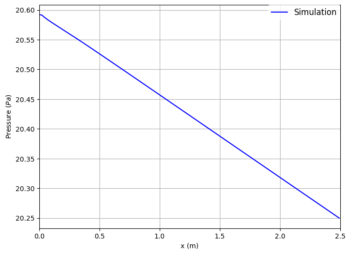
To create these plots, run python plot_track.py to create the plots. Before running the plot script, open 'plot_track.py' and update path to Gleaner script in 'glrPath'. Download Gleaner script using hg clone https://geb.inf.tu-dresden.de/hg/gleaner.